DE ANATOMÍA PATOLÓGICA
| IV CONGRESO VIRTUAL HISPANOAMERICANO DE ANATOMÍA PATOLÓGICA |
|
Versión con imágenes ampliadas (1.312 KB) |
Abstract:
Electronic noise is ubiquitous to any digital image. When procuring images there is a random variation of pixels values within regions of the image that they are uniform in the original scene due to limited detection or counting of incident photons or due to interference from amplifiers, cabling and background light. Such interference is referred to as electronic "noise". The ratio of the number of photons recorded by the CCD (signal) to the noise which is due to structural differences in the CCD and other components of the imaging system refers as to, signal-to-noise ratio (S/N). The higher this ratio the better the image. Even after constant illumination the exact number of photons recorded is unpredictable due to variations in the electronic noise.
All digital images have a certain amount of electronic noise. When noise is perceived by the human eye the amount of noise is significant and detracts from the way the image looks. Then, it is time to use imaging tools to reduce the amount of noise and hence improve the image looks.
This presentation includes a series of digital pictures representing several difficult ultrasound guided prostatic lesions from five patients. The images were all obtained in one single session with the same equipment and were all jpeg with the same compression ratio. All these images exhibit visually detectable noise of various kinds. Detectable noise is particularly noticeable at 200% enlargements or higher. With the use of image processing tools (PhotoShop) it is possible to apply algorithms that reduce electronic noise and enhances the quality of these images.
Detailed steps using PhotoShop are described to reduce noise and improve the quality of digital images with various degrees and kinds of electronic noise. Specific guidance on how to minimize noise when procuring digital images is discussed in detail in this presentation.
Key Words: Electronic Noise, Digital Images, Prostatic Carcinoma,
Electronic noise can be defined as a distortion of an image's analog signal. It is an analog problem that is confined to the analog electronics of scanning device or sensor. Once a signal is digitized, if it stored in a lossless file format it is relatively immune to noise. Electronic noise is ubiquitous to any digital image. Noise maybe random or periodic. Random noise usually occurs in the spatial domain of images. It is the random distortion in an analogue signal causing snow or speckles (random spots) throughout the image. The distortion can be the result of electronic noise in the amplifiers, electrical spikes somewhere in the system, or random fluctuations in the source lights. Periodic noise takes place in the frequency domain of images. It is a recognizable pattern of change in an image file. The change is an increase or a decrease in the brightness of the pixels compared to what they should be. The pattern can be horizontally across a raster line, vertically down through the raster lines, or diagonal
ly down and across the raster lines. Vertical correlated noise is often called streak noise and is a common problem with CCD technology. In this presentation I will be addressing the electronic noise that can be modify in the spatial domain of images.
All CCD cameras are produce electronic noise: dark noise and read-out-noise. Dark noise is visible as "white pixels" within an image. Reducing the temperature at which the CCD operates can minimize it. Read-out-noise is generated by the A/D converter, which amplifies and transforms the charge accumulated by each photodiode when stricken by incident photons.
When procuring images there is a random variation of pixels values within regions of the image that they are uniform in the original scene due to limited detection or counting of incident photons or due to interference from amplifiers, cabling, background light or other electric interference.
The ratio of the number of photons recorded by the CCD (signal) to the noise which is due to structural differences in the CCD and other components of the imaging system refers as to, signal-to-noise ratio (S/N). The higher this ratio the better the image. Even after constant illumination the exact number of photons recorded is unpredictable due to variations in the electronic noise.
Stray light arises from room light particularly fluorescence light or sources within the microscope. Photon statistical noise originates from photon statistics and it is added to statistical electronic noise generated in the video camera. It is inherent to the signal and can be reduced by frame averaging and cooling the CCD.
Other cases of electronic noise is generated by electric AC tools or appliances, which generate low frequencies than can be pickup by connecting cables in the system acting as an antenna.
Other source of noise refers to optical noise produced by any of the optical parts of the microscope. Dirt, dust particles, lint, or smears of oil in the glass slides or the lenses of the microscope will introduce electronic noise in the digitized image.
Additional sources of optical noise are: stray light and photon statistical noise.
Another overlooked source of noise in digital images is processing noise. Processing jpeg digital images introduces "new pixels" in the image each time than a jpeg image is saved by the image processing program resulting in progressing degradation of the image and adding processing noise.
Since electronic noise is ubiquitous it is understandable that all digital images bear a certain amount of noise. By its very nature, noise causes the values of adjacent pixels to be different even if they were illuminated identically during an exposure. When noise is perceived by the human eye the amount of noise is significant and detracts from the way the image looks. Then, it is time to use imaging tools to reduce the amount of noise and hence improve the image looks.
A Sony (Sony Corp.) analog camera, Snappy V. 1.0 (Play Inc.), PhotoShop V. 5.5 (Adobe Inc.). H & E slides from five cases of USGPNB biopsies. Figures are jpeg. Avoid changing magnification or saving them again under jpeg. Use screen displays of 640x480 or 1022x768. You will have to download the images from the Congress site to really appreciate the difference between the left and the right side of each figure after zooming in to about 200-300%.
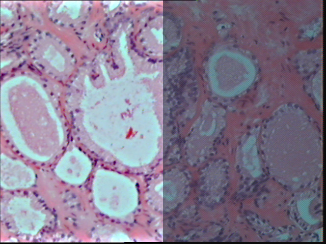
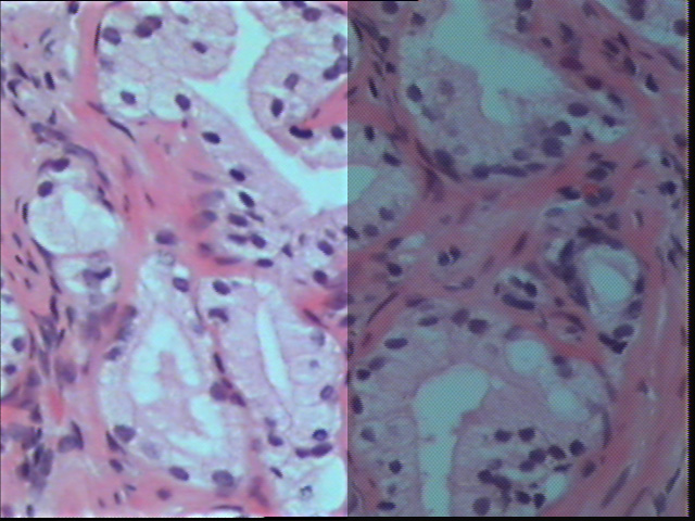
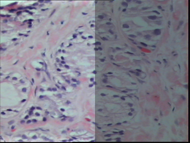 (Pulse sobre la imagen para ampliarla) (Pulse sobre la imagen para ampliarla)Figure 1: Ultrasound guided prostatic needle biopsy (USGPNB). H&E section of small adenocarcinoma of prostate, Gleason 3+3.
This image shows several problems. On high magnification (200%-400%) noise is very apparent in the right side of the image. In addition the image is too dark.
The left half side of the image was selected with the rectangular marquee tool in PhotoShop 5.5. Zoom in to about 300%, to see the ragged (noisy) background.
Go to Filter -> Noise -> Despeckle. Notice the difference. After that, go to Filter -> Sharpen -> Unsharp Mask, and use 50%, 15 radius and 3 threshold. Notice the difference. Go to Image -> Adjust -> Levels, and adjust the RGB histogram by moving the left, right and middle arrows. Zoom out to 100%. Notice the difference between the left and the right side of the image.
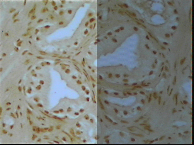
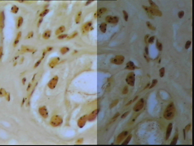 (Pulse sobre la imagen para ampliarla) (Pulse sobre la imagen para ampliarla)Figure 2: Same case as Figure 1. Silver stain for Nucleolar Organizer Regions (AgNOR'S).
This image shows also noise more apparent at enlargements of 200%-400%. It is also too dark. Poor illumination may have played a role in the noisy background. Jpeg compression is probably responsible for some of the background noise.
The left side of the image was again selected for comparison, with the rectangular marquee tool. Zoom in to about 300%, to see the geometric (noisy) background. Go to Filter -> Noise -> Despeckle. Notice the difference. After that, go to Filter -> Sharpen -> Unsharp Mask, and use 50%, 15 radius and 3 threshold. Notice the difference. Go to Image -> Adjust -> Levels, and adjust the RGB histogram by moving the left, right and middle arrows. Zoom out to 100%.
Notice the difference.
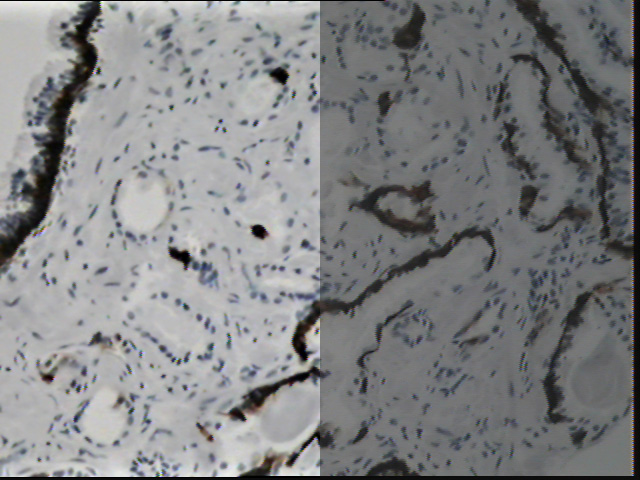
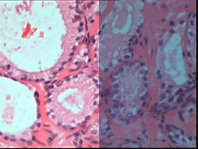
 (Pulse sobre la imagen para ampliarla) (Pulse sobre la imagen para ampliarla)Figure 3: Ultrasound guided prostatic needle biopsy (USGPNB). H&E section. A consultant called this small lesion: "suspicious but not diagnostic for carcinoma".
This image shows also noise more apparent at enlargements of 200%-400%. It is also too dark.
The left side of the image was again selected for comparison, with the rectangular marquee tool. Zoom in to about 300%, to see the ragged (noisy) background. Go to Filter -> Noise -> Despeckle. Notice the difference. After that, go to Filter -> Sharpen -> Unsharp Mask, and use 50%, 15 radius and 3 threshold. Notice the difference. Go to Image -> Adjust -> Levels, and adjust the RGB histogram by moving the left, right and middle arrows. Zoom out to 100%.
 (Pulse sobre la imagen para ampliarla) (Pulse sobre la imagen para ampliarla)Figure 4: Same case as figure 3. High molecular keratin staining for basal layer. Some glands lack a basal layer.
Again, The left side of the image was again selected for comparison, with the rectangular marquee tool. Zoom in to about 300%, to see the ragged (noisy) background. Go to Filter -> Noise -> Despeckle. Notice the difference. After that, go to Filter -> Sharpen -> Unsharp Mask, and use 50%, 15 radius and 3 threshold. Notice the difference. Go to Image -> Adjust -> Levels, and adjust the RGB histogram by moving the left, right and middle arrows. Zoom out to 100%.
 (Pulse sobre la imagen para ampliarla) (Pulse sobre la imagen para ampliarla)Figure 5: Ultrasound guided prostatic needle biopsy (USGPNB). H&E section. A consultant called this small lesion: "Atypical, suspicious but not diagnostic for carcinoma".
Again, The left side of the image was again selected for comparison, with the rectangular marquee tool. Zoom in to about 300%, to see the ragged (noisy) background. Go to Filter -> Noise -> Despeckle. Notice the difference. After that, go to Filter -> Sharpen -> Unsharp Mask, and use 50%, 15 radius and 3 threshold. Notice the difference. Go to Image -> Adjust -> Levels, and adjust the RGB histogram by moving the left, right and middle arrows. Zoom out to 100%.
 (Pulse sobre la imagen para ampliarla) (Pulse sobre la imagen para ampliarla)Figure 6:
Same case as figure 5. H&E section. Higher magnification of same field.
Again, The left side of the image was again selected for comparison, with the rectangular marquee tool. Zoom in to about 300%, to see the ragged (noisy) background. Go to Filter -> Noise -> Despeckle. Notice the difference. After that, go to Filter -> Sharpen -> Unsharp Mask, and use 50%, 15 radius and 3 threshold. Notice the difference. Go to Image -> Adjust -> Autolevels. Zoom out to 100%.
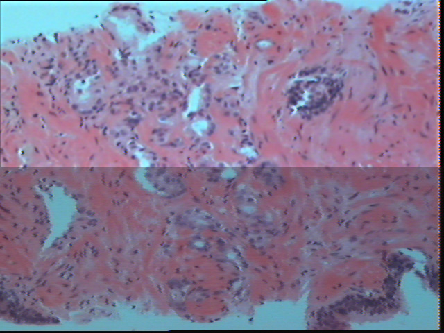 (Pulse sobre la imagen para ampliarla) (Pulse sobre la imagen para ampliarla)Figure 7: Ultrasound guided prostatic needle biopsy (USGPNB). H&E section. Again another contraversial lesion. A consultant called this small lesion: "Atypical, suspicious but not diagnostic for carcinoma".
Again, The top of the image was again selected for comparison with the bottom, with the rectangular marquee tool. Zoom in to about 300%, to see the ragged (noisy) background. Go to Filter -> Noise -> Despeckle. Notice the difference. After that, go to Filter -> Sharpen -> Unsharp Mask, and use 50%, 15 radius and 3 threshold. Notice the difference. Go to Image -> Adjust -> Levels, and adjust the RGB histogram by moving the left, right and middle arrows. Zoom out to 100%.
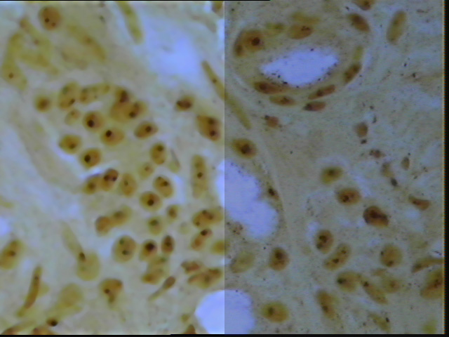 (Pulse sobre la imagen para ampliarla) (Pulse sobre la imagen para ampliarla)Figure 8:Same case as figure 7. Silver stain for Nucleolar Organizer Regions (AgNOR'S). The background shows silver precipitate (technical noise) in addition to electronic noise.
Again, The left side of the image was again selected for comparison, with the rectangular marquee tool. Zoom in to about 300%, to see the ragged (noisy) background. Go to Filter -> Noise -> Dust&Scratches, use a radius of about 3 and threshold of 1. Notice the difference. After that, go to Filter -> Sharpen -> Unsharp Mask, and use 50%, 15 radius and 3 threshold. Notice the difference. Go to Image -> Adjust -> Levels, and adjust the RGB histogram by moving the left, right and middle arrows. Zoom out to 100%.
 (Pulse sobre la imagen para ampliarla) (Pulse sobre la imagen para ampliarla)Figure 9: Same case as figure 7. High molecular keratin staining for basal layer. Many glands lack a basal layer.
Again, The top of the image was again selected for comparison with the bottom, with the rectangular marquee tool. Zoom in to about 300%, to see the ragged (noisy) background. Go to Filter -> Noise -> Despeckle. Notice the difference. After that, go to Filter -> Sharpen -> Unsharp Mask, and use 50%, 5 radius and 3 threshold. Notice the difference. Go to Image -> Adjust -> Autolevels. Zoom out to 100%.
 (Pulse sobre la imagen para ampliarla) (Pulse sobre la imagen para ampliarla)Figure 10: Ultrasound guided prostatic needle biopsy (USGPNB). H&E section. A consultant called this small lesion: "Benign, acinar atrophy"
Again, The left side of the image was again selected for comparison, with the rectangular marquee tool. Zoom in to about 300%, to see the ragged (noisy) background. Go to Filter -> Noise -> Despeckle. Notice the difference. After that, go to Filter -> Sharpen -> Unsharp Mask, and use 50%, 15 radius and 3 threshold. Notice the difference. Go to Image -> Adjust -> Levels, and adjust the RGB histogram by moving the left, right and middle arrows. Zoom out to 100%.
 (Pulse sobre la imagen para ampliarla) (Pulse sobre la imagen para ampliarla)Figure 11: Same case as figure 10. Silver stain for Nucleolar Organizer Regions (AgNOR'S).
The left side of the image was again selected for comparison, with the rectangular marquee tool. Zoom in to about 300%, to see the geometric (noisy) background. Go to Filter -> Noise -> Despeckle. Notice the difference. After that, go to Filter -> Sharpen -> Unsharp Mask, and use 50%, 15 radius and 3 threshold. Notice the difference. Go to Image -> Adjust -> Levels, and adjust the RGB histogram by moving the left, right and middle arrows. Zoom out to 100%.
Notice the difference.
Snappy was one of the first digitizer-framegrabber cards for PC computers. Snappy can take the input of an NTSC video is or an analog signal and converted into a 24 bit digital image. Its chip samples each analog line up to 1500 times therefor improving the image capture by frame averaging. The software includes time base correction, spatial and temporal filters and image interpolation that converts 480 lines tall NTSC video vertically to maintain square pixels. A nine-volt battery powers the device. Snappy however is not a perfect digitizing card and under certain conditions it can produce images with significant amount of noise.
Analog cameras have inherent limitations. When used in electrically noisy environments where data rates can exceed 100MB's per second the signal sensitivity to noise rises exponentially. Digital cameras where the digitization is performed in the camera it self as opposed to using a digitization card with an analog camera significantly diminishes the noise sensitivity and improves the signal. Since the cost of digital cameras is rapidly dropping the trend is to use digital cameras as opposed to analog cameras.
As I have shown digital images presented contained noise of various kinds. Most image processing tasks are considerably simplified if this noise can be removed.
A general approach to noise removal is to smooth the image by replacing each pixel value by a new value, which is a function of the values in some neighborhood of the pixel.
This is usually accomplished with a low-pass filter. Sometimes called blurring or smoothing, low-pass filtering averages out rapid changes of intensity from one pixel to the next. For example, a simple low-pass filter might replace a pixel's value with the average of its original value and that of its eight surrounding neighbors. This process is repeated for each pixel in the image, and the result looks blurrier than the original. Since details we are trying to record are usually spread across many adjacent pixels, and the value of one pixel is related to the value of its neighbors. Thus, the averaging effect of a low-pass filter influences the random noise more than it does the image. Suppressing noise helps reveal gradual background changes that might otherwise be invisible.
By changing the convolution kernel the final value for the pixel at the kernel's center is changed thus you can experiment with different low-pass filters. The functions in PhotoShop of Despeckle and Dust&Scratches are basically low-pass filters.
The Unsharp Mask filter will enhance your image by making it sharper without accentuating the small imperfections in the image. Unsharp Mask is based on a darkroom technique that was used before computer graphics arrived on the scene. It is a very efficient filter for sharpening enhancements. A low-pass filter is first used to make a blurry copy of the original image. This copy is subtracted from the original, suppressing large-scale features and leaving fine detail. A one-for-one subtraction usually has much too harsh an effect, but the amount of filtering is easily adjusted. For example, before subtraction, we can multiply each pixel in the original image by 3 and each pixel in the copy by 2. The resulting image has some large-scale features remaining, while small-scale features are amplified. With this technique the amount of enhancement can be easily controlled to get the best effect
To increase contrast, usually, it's much better to use Unsharp Mask than Sharpen function. The reason for this is that Unsharp Mask will sharpen the edges in the image, and the human eye is very sensitive to "unsharp" edges. Actually, sharpening the edges in an image will make the whole image look sharp, because you will not easily detect the other parts that are less sharp. Also, because Unsharp Mask won't sharpen the entire image as much as the Sharpen filter does, the resulting image will look much more natural than the somewhat artificial look that Sharpen will produce.
Another function used in this presentation, levels was used to stretch or expand the histogram of an acquired digital image. The following is a rationalization of how it works.
Many CCD cameras can differentiate 256 levels of brightness (8-bit data). Any acquired digital image, including the figures included in these presentation have a unique histogram usually significantly less than 256 levels of brightness. You can visualize this histogram by using the function levels, in PhotoShop. It function represents a numeric graphic display of every pixel value. The larger the number, the brighter the pixel. When adjusting the left and right arrows you are defining the unique dynamic range for each image. The program stretches an image by modifying every pixel value with a simple mathematical formula.
The best results are usually attained by manually tweaking the numbers based on the brightest and dimmest pixels in each image.
There are many variables that you can experiment and try. The main problem with stretching is to decide which features are the ones you want to emphasize and then to determine precisely how to adjust the pixel brightness for best effect.
Guidelines to minimize electronic noise: 1.- Use a digital camera if your budget permits, instead an analog camera. Regardless which camera you choose, select one with a CCD chip has the best possible Dynamic Range. This range is closely related to the signal-to-noise ratio. It is measured in Decibels (dB). The higher the decibels the better. 2.- Pay good attention to illumination and color temperature of the light source. Good sources and detail to illumination will make a big difference in obtaining the best possible digital image. When procuring a digital image from a gross specimen consider a "ring" flash attached to the camera. When using a microscope on low magnifications remember to flip out the condenser. 3.- Avoid cabling crossing particularly with power cables. 4.- Avoid possible sources of electric or electronic of noise in the environment. 5.- If you use jpeg compressed image files always save the original file in a lossless image format (Tiff). Do your processing steps with the original file and save the modifications in a jpeg-compressed format. Minimize "jpegging" an image more than once. 6.- Examine digital images at 200%-300% magnification and if noise is apparent consider reducing it with some the techniques discussed in this presentation. Mariano Alvira, MD, LifeSpan Biosciences Inc., Seattle, WA, USA alviram@altavista.com
|